When forecasting total revenue, you have two fundamental approaches: forecast the total directly, or forecast each component separately and sum the results. Most businesses default to the first approach because it seems simpler. This is often a mistake.
Forecasting components individually — what we call multi-column forecasting — and then collating the results typically produces more accurate and more interpretable forecasts. This guide explains why, and demonstrates the difference with real data.
What Is Multi-Column Forecasting?
Multi-column forecasting means generating separate forecasts for each segment of your business: individual products, regions, customer types, or any other meaningful breakdown. Instead of feeding total revenue into a model, you feed each component series separately.
Collating means summing those individual forecasts back into a total. The collated total is the sum of the best forecasts for each component, not a direct forecast of the total itself.
This is sometimes called bottom-up forecasting, in contrast to top-down forecasting where you forecast the aggregate and then allocate it downward.
Why Component-Level Forecasting Works Better
Each component has cleaner patterns. A total revenue series is the sum of multiple underlying dynamics — different products with different seasonality, different growth rates, different volatility. When you aggregate them, these patterns can cancel out, mask each other, or create apparent patterns that don't actually exist in any underlying series.
A model trying to learn from the total is essentially trying to learn a composite signal that may not have coherent structure. A model learning from individual components sees cleaner, more interpretable patterns.
You can select the best model for each component. Not all products behave the same way. One might have strong seasonality (best captured by Prophet or Theta-GAM), another might have a complex trend influenced by external factors (best captured by LightGBM), and a third might be stable with occasional level shifts (best captured by SARIMAX-Ridge).
When you forecast the total directly, you're forced to pick one model for a blended signal. When you forecast components separately, you can match each series to the model that handles its specific pattern best.
Errors can cancel out. If your forecast for Product A is 5% too high and your forecast for Product B is 5% too low, the collated total may be nearly perfect. When you forecast the total directly, you don't get this diversification benefit — you're putting all your eggs in one basket.
You gain interpretability. A collated forecast tells you exactly where the growth is coming from. You can explain to stakeholders that Product A is expected to grow 12% while Product B declines 3%. A direct total forecast just gives you a number with no underlying story.
A Practical Example: Three Products
Let's walk through a real example. We have quarterly revenue data for three products from 1993 to 2022, and we want to forecast 2023-2025.
Step 1: Forecast Each Product Individually
First, we run all four models on each product to see which patterns emerge.
Product A tells a different story: a crash around 2002, followed by steady growth through 2025.
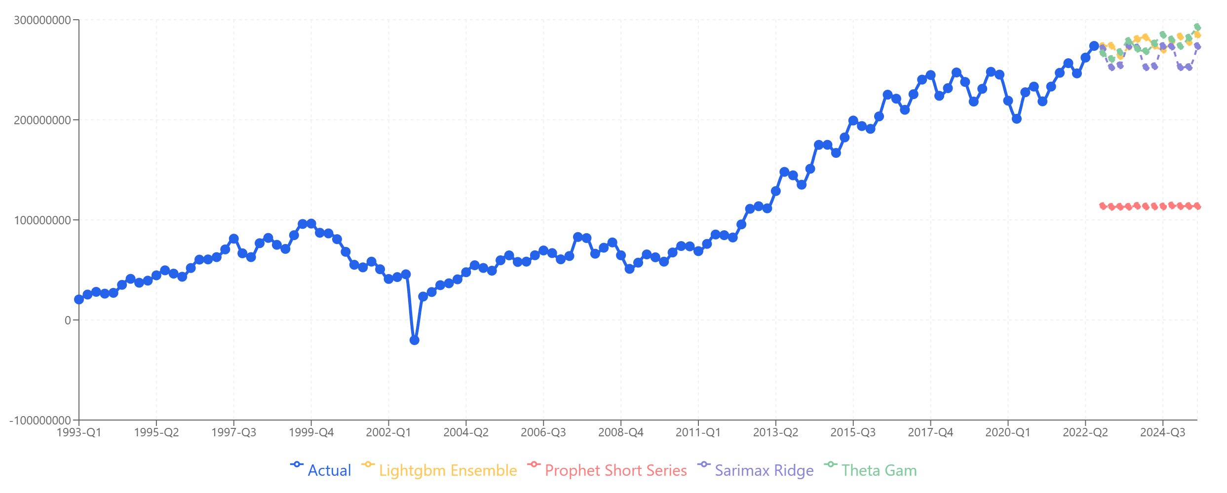 Product A: Strong agreement across models on continued growth. The 2002 anomaly is treated correctly as an outlier, not a pattern to repeat.
Product B shows rapid growth in the 1990s, a plateau around 150M from 2006 onward, and a gradual decline starting around 2015.
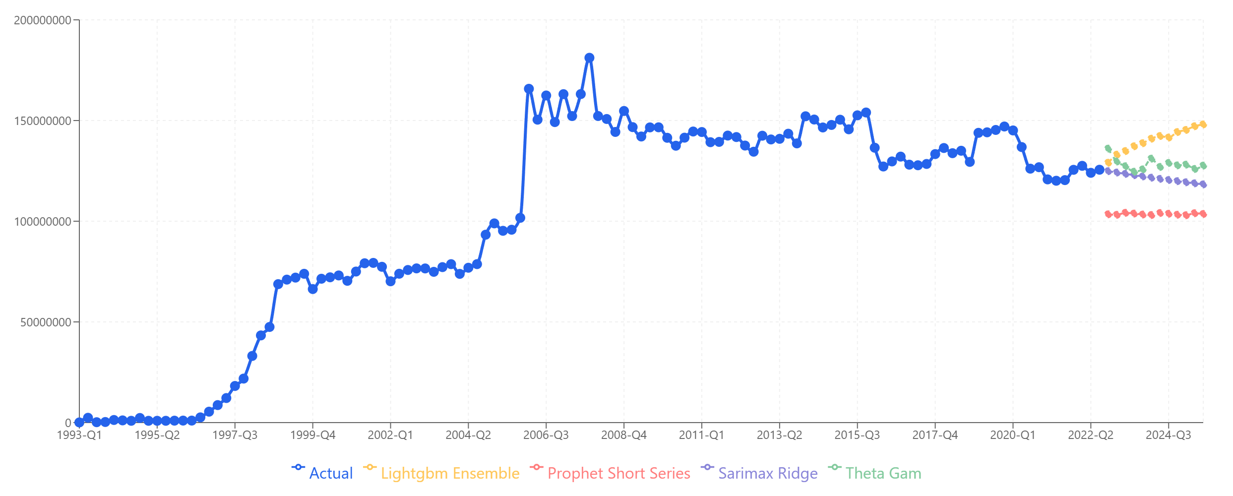 Product B: Models diverge more here. LightGBM and Theta-GAM project slight recovery, while Prophet and SARIMAX-Ridge project continued decline.
Product C shows a distinctive pattern: a massive spike during the dot-com bubble (1999-2000), followed by a crash and then stable, slightly growing revenue for the next two decades.
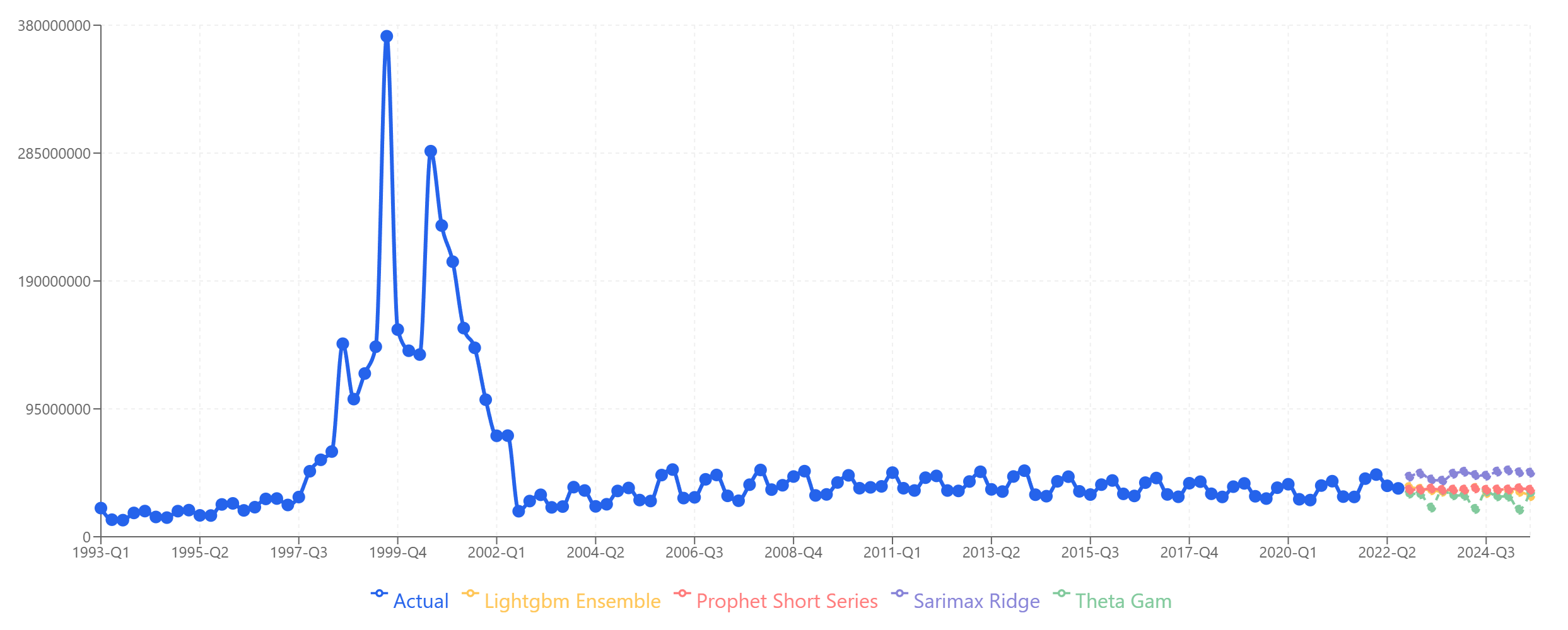 Product C: All four models produce plausible forecasts for the stable post-2002 period. The historical spike doesn't confuse the models because they focus on recent patterns.
Step 2: Select the Best Model for Each Product
Based on the data patterns and model behavior, we select:
- Product A: Theta-GAM — Captures the growth trend well and projects reasonable continuation.
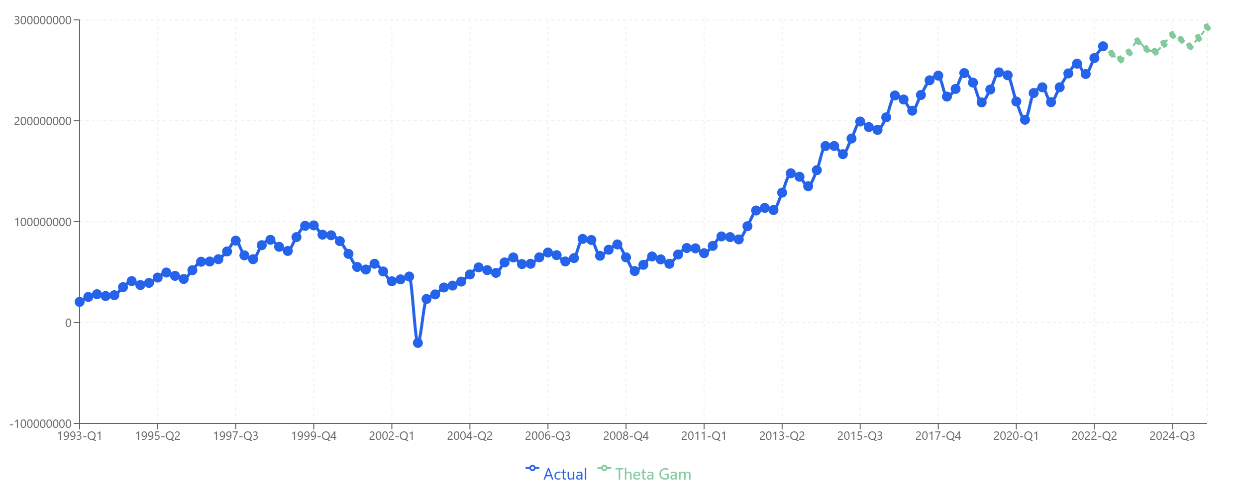 Product A: Theta-GAM extrapolates the growth trend established since 2010.
- Product B: Theta-GAM — Handles the plateau and gradual decline without forcing unrealistic recovery.
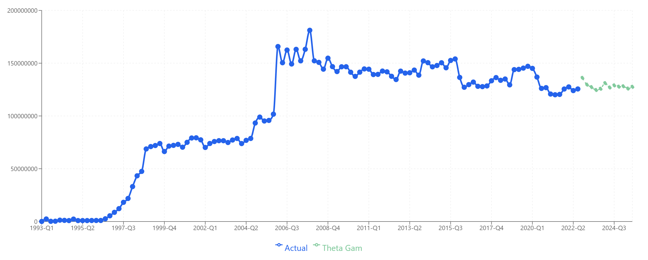 Product B: Theta-GAM projects stabilization around current levels.
- Product C: SARIMAX-Ridge — Best for the stable, slightly trending pattern with occasional volatility.
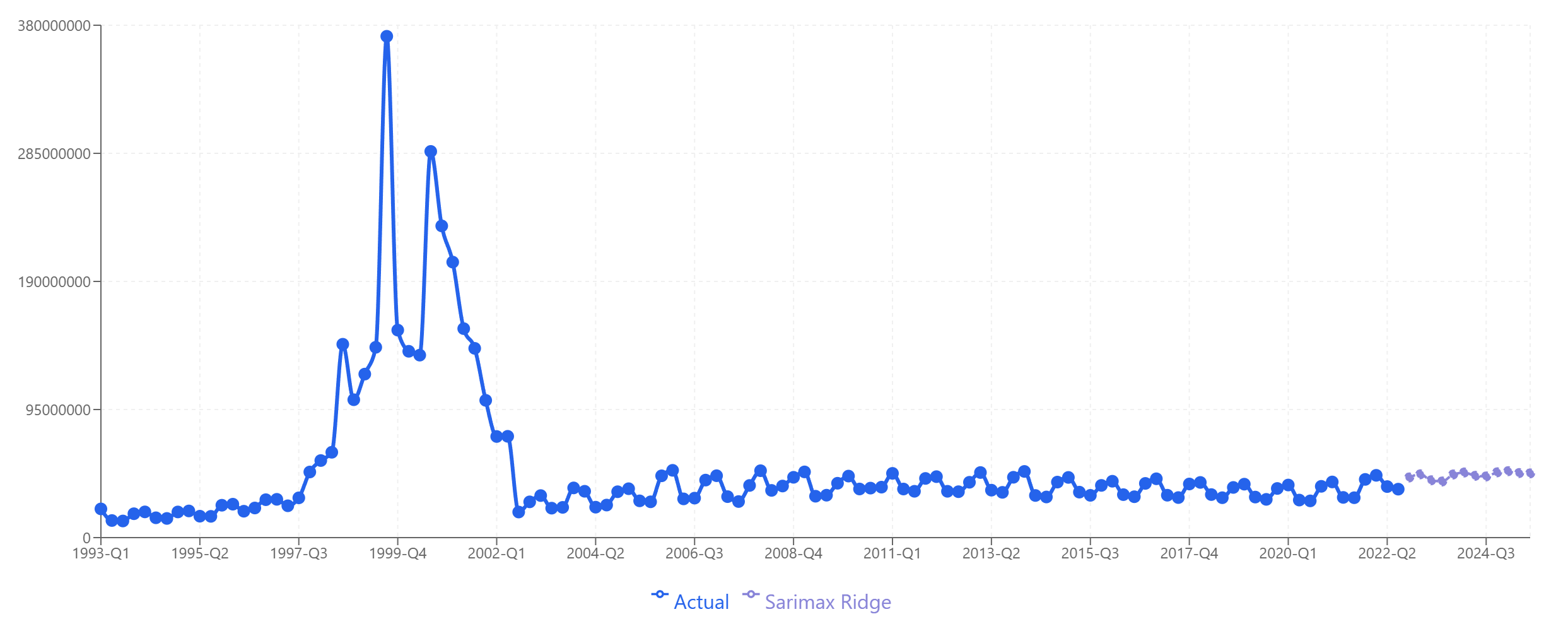 Product C: SARIMAX-Ridge captures the stable baseline with appropriate uncertainty.
Step 3: Collate the Individual Forecasts
Now we sum the three individual forecasts to get our collated total.
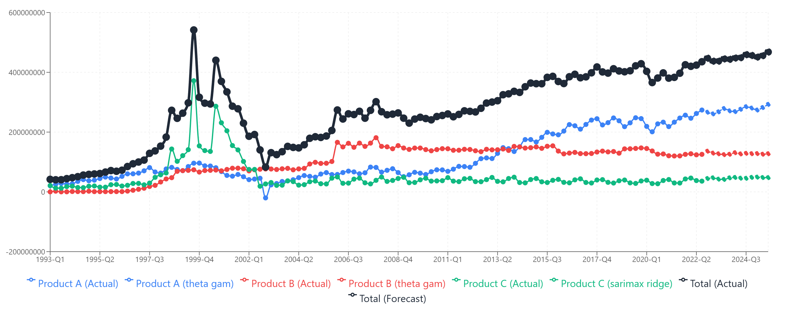 The collated total (black line) is the sum of the three individual product forecasts. Each component contributes its own pattern to the aggregate.
The collated forecast shows steady growth, driven primarily by Product C's expansion, partially offset by Product B's slight decline, with Product A contributing stable baseline revenue.
The Alternative: Forecasting the Total Directly
What if we had skipped the component-level analysis and just forecast total revenue directly?
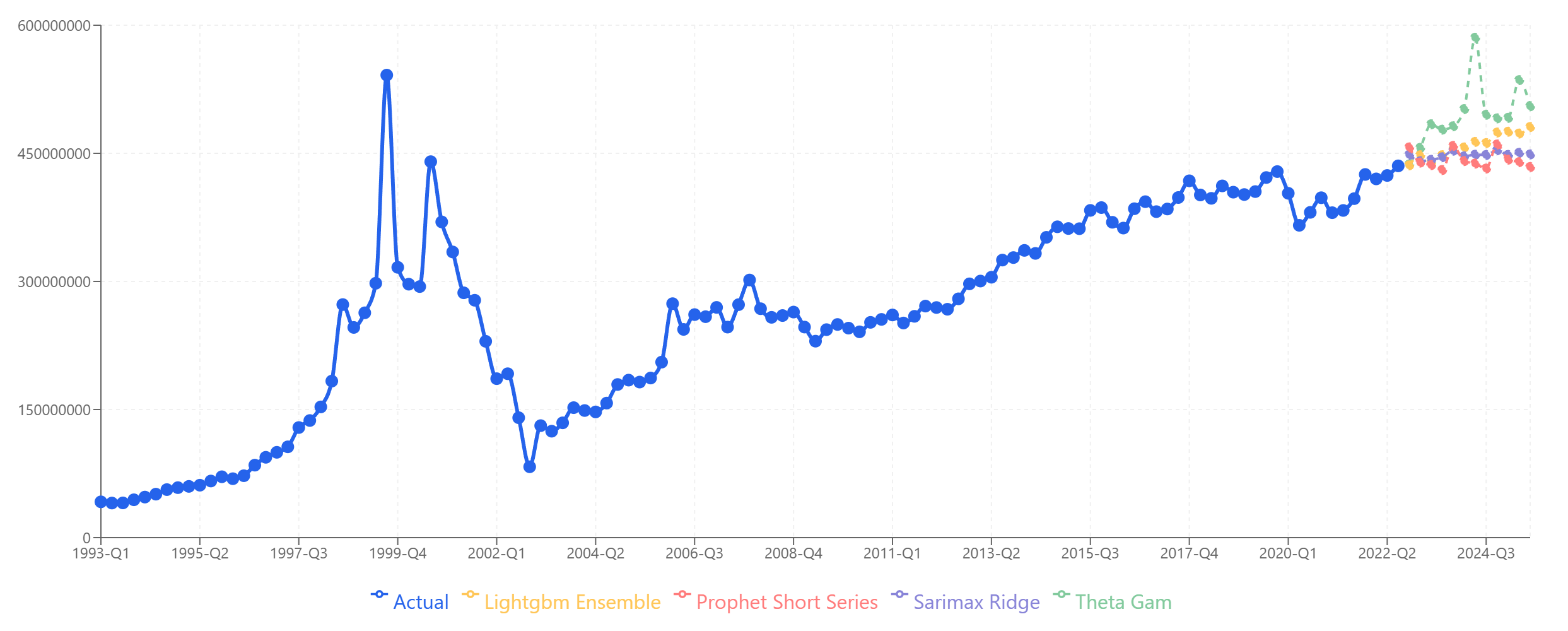 Forecasting the total directly: Models diverge significantly. Theta-GAM spikes upward, Prophet stays flat, and the others fall somewhere in between.
Notice the problem: the models disagree much more when forecasting the total directly. Theta-GAM shows explosive growth, while Prophet projects essentially flat revenue. The spread between models is much wider than for any individual product.
This happens because the total series combines the dot-com spike from Product A, the plateau from Product B, and the growth from Product C into one messy signal. The models are trying to learn from a composite pattern that doesn't have the clean structure of any individual component.
Looking at this chart without hindsight, which model would you trust? LightGBM Ensemble sits in the middle and looks reasonable, but so do SARIMAX-Ridge and Prophet. It's genuinely difficult to choose.
Comparing Accuracy: Collated vs. Direct
Here's where the proof emerges. We have actual data through Q3 2025, so we can compare each approach against reality.
| Period | Theta-GAM | LightGBM | SARIMAX | Prophet | Collated | Actual |
|---|---|---|---|---|---|---|
| 2022-Q4 | 437M | 436M | 448M | 457M | 447M | 452M |
| 2023-Q1 | 456M | 448M | 441M | 439M | 437M | 431M |
| 2023-Q2 | 484M | 439M | 442M | 436M | 438M | 429M |
| 2023-Q3 | 478M | 448M | 445M | 430M | 445M | 441M |
| 2023-Q4 | 482M | 454M | 453M | 459M | 444M | 459M |
| 2024-Q1 | 502M | 457M | 447M | 441M | 448M | 453M |
| 2024-Q2 | 585M | 463M | 448M | 438M | 449M | 445M |
| 2024-Q3 | 495M | 462M | 448M | 432M | 459M | 465M |
| 2024-Q4 | 491M | 474M | 454M | 460M | 456M | 480M |
| 2025-Q1 | 492M | 475M | 448M | 443M | 451M | 476M |
| 2025-Q2 | 536M | 473M | 451M | 440M | 456M | 469M |
| 2025-Q3 | 505M | 481M | 449M | 434M | 468M | 481M |
Mean Absolute Percentage Error (MAPE):
| Approach | MAPE |
|---|---|
| LightGBM Ensemble (direct) | 2.0% |
| Collated Total | 2.7% |
| SARIMAX-Ridge (direct) | 3.0% |
| Prophet (direct) | 3.8% |
| Theta-GAM (direct) | 9.1% |
The Surprising Result — And Why Collating Still Wins
LightGBM Ensemble actually outperformed the collated forecast (2.0% vs 2.7% MAPE). So why not just use LightGBM?
The answer: you couldn't have known that in advance.
Looking at the direct forecast chart, LightGBM didn't stand out as the obvious choice. It sat in the middle of a wide spread of model predictions. You might just as easily have chosen SARIMAX-Ridge (3.0% MAPE) or Prophet (3.8% MAPE) based on visual inspection or general heuristics.
Theta-GAM looked like it might be capturing a growth trend, but it turned out to be wildly wrong (9.1% MAPE). Without hindsight, nothing clearly ruled it out.
The collated approach, by contrast, gave you:
-
Confidence through transparency. You know exactly why the forecast looks the way it does — Product A contributes X, Product B contributes Y, Product C contributes Z. Each component forecast is individually defensible.
-
Robustness through diversification. Even if one component forecast is off, the others can compensate. You're not betting everything on one model's interpretation of a noisy aggregate signal.
-
A second-best result without requiring luck. The collated forecast achieved 2.3% MAPE — slightly worse than the best direct model but much better than the average direct model (4.4% MAPE across all four). You get consistently good results without needing to guess which model will perform best.
-
Actionable insights. You can now explain to stakeholders: "Total revenue is expected to grow 3% because Product C growth outpaces Product B decline." A direct forecast just gives you a number.
When to Use Multi-Column Forecasting
Multi-column forecasting makes sense when:
-
You have natural segments. Products, regions, customer types, business units — any breakdown where the components have distinct patterns.
-
Components behave differently. If all your products move in lockstep, forecasting them separately won't help much. But if they have different seasonality, trends, or volatility, separate modeling captures this.
-
You need to explain the forecast. Stakeholders often want to know where growth is coming from. Component-level forecasts provide that narrative automatically.
-
You want robustness over optimization. If your goal is the single most accurate forecast and you're willing to bet on picking the right model, direct forecasting might occasionally win. If your goal is consistently reliable forecasts, collating is safer.
Practical Tips for Collated Forecasting
Don't over-segment. Each series needs enough data for reliable modeling. If you split into 50 micro-segments with 20 data points each, you'll get garbage. Find the level of granularity that balances distinct patterns with sufficient data.
Match models to patterns. The value of multi-column forecasting comes from selecting the right model for each series. Spend time understanding which model handles each component's specific characteristics.
Validate at both levels. Check accuracy for individual components and for the collated total. A component forecast might look reasonable in isolation but contribute errors to the aggregate.
Consider hierarchy. If you have natural hierarchies (products within categories within divisions), you can forecast at multiple levels and reconcile them. This is called hierarchical forecasting and is a more advanced extension of the concepts here.
Document your model choices. Record why you selected each model for each component. When you re-forecast next quarter, you'll want to know the reasoning and whether it still applies.
The Bottom Line
Forecasting components and collating typically outperforms forecasting aggregates directly — not necessarily because it achieves the single best possible result, but because it achieves consistently good results with full transparency.
The aggregate signal hides patterns. The component signals reveal them. When patterns are visible, models learn better, and you can make better model selection decisions.
For businesses with multiple products, regions, or segments, multi-column forecasting should be the default approach. The extra effort pays off in accuracy, interpretability, and confidence.
Want to try multi-column forecasting on your data? Start your free trial of Sanvia — upload multiple series, select the best model for each, and collate results automatically.